2024년 4월 11일 목요일

도커 이미지 빌드 시 문제 해결 솔류션 정리

이 글은 도커 이미지 빌드 시 문제 해결 솔류션을 정리한 글이다. 


도커 컨테이너 이미지는 개발, 운영 환경을 독립적으로 실행할 수 있는 가상화를 지원한다. 다만, 도커 이미지 빌드 시 설치되는 수많은 패키지에 의존되므로, 여러 에러가 발생된다. 대표적인 에러는 다음과 같다. 
  1. 'DEBIAN_FRONTEND=noninteractive' not working inside shell script with apt-get
  2. How can I set the default timezone
  3. Docker build failed with Hash Sum mismatch error
  4. Docker build failed with error "Hash Sum mismatch"
  5. throws an error saying "Some index files failed to download. They have been ignored or old ones used instead."
  6. Error while loading conda entry point: conda-libmamba-solver (libarchive.so.19: cannot open shared object file: No such file or directory)
  7. OpenGL, 3D graphics problems in docker
  8. Windows Volume mount
이외에도 매우 다양한데, 사실, 설치되는 패키지들이 많은 도커 이미지는 그만큼 원인이 많다. 스택 오버플로우 관련 댓글을 보면 알겠지만, 누구는 이런 문제로 몇 일이 날라갔다 등의 성토글을 볼 수 있다. 그만큼 원인이 다양하게 조합될 수 있다.

앞의 에러 솔류션만 정리해 본다. 

1번은 도커 빌드 시 [yes/no] 프롬프트 입력 상황에서 발생한다. 도커 빌드 중에는 키보드 입력이 안된다. 그러므로, 다음과 같이 인터렉티브가 없다고 설정하면 해결된다.
ARG DEBIAN_FRONTEND=noninteractive

2번은 타임존 문제로 이는 다음과 같이 설정한다. 타임존이 제대로 설정되어 있지 않으면, 패키지 설치에 실패할 수 있다. 
ENV LANG=C.UTF-8 LC_ALL=C.UTF-8
ENV TZ=Asia/Seoul

3, 4번 해쉬섬 에러 문제는 보통 우분투나 리눅스의 apt-get update 시 발생하는 데, stack overflow에 검색해 보아도 관련 솔류션을 시도해도 잘 처리 안되는 경우가 발생한다. 

이 경우는 다음과 같은 솔류션을 apt-get update 전에 dockerfile에 정의하라고 되어 있는 답변이 많다. 

RUN rm -rf /var/lib/apt/lists/*

RUN echo "Acquire::http::Pipeline-Depth 0;" > /etc/apt/apt.conf.d/99custom && \
    echo "Acquire::http::No-Cache true;" >> /etc/apt/apt.conf.d/99custom && \
    echo "Acquire::BrokenProxy    true;" >> /etc/apt/apt.conf.d/99custom

RUN echo "Acquire::Check-Valid-Until \"false\";\nAcquire::Check-Date \"false\";" | cat > /etc/apt/apt.conf.d/10no--check-valid-until

이렇게 해도 해결안되면, 기본이 되는 이미지를 우분투 과거 버전(예. 20.04), 혹은 미리 패키지 설치된 버전으로 설정하고 다시 시도한다. 
FROM ubuntu:20.04
FROM continuumio/miniconda3

이 문제는 무언가 해당 패키지를 배포하는 서버에서 문제가 있거나, 도커 빌드 컴퓨터의 시간이 안맞는 등의 문제로 예상된다. 

5번은 도커 이미지 빌드 시 동작되는 방식에 원인이 있다. 도커는 빌드 과정을 재활용하기 위해 레이어, 캐쉬 등을 사용하는 데, 가끔 이 부분이 꼬이는 경우가 있다. 이 경우, 다음과 같이 빌드해 본다 .
docker build --no-cache -t <docker_name> .

안되면, 현재 도커 이미지들을 모두 삭제하거나, 다음과 같이 clean, purge를 한다.
docker image rm -f
docker system prune -a -f

6번은 미리 설치된 아나콘다 이미지를 사용하라고 권장한다. 다음은 그 예이다.
FROM continuumio/miniconda3

7번은 호스트 서버가 3D GPU가 지원되지 않으면 아직 뚜렷한 해결방법은 없다. 도커 이미지는 본질적으로 3D GUI용으로 사용되도록 개발된 것이 아니다. 3D GUI로 이미지를 생성, 저장하는 등의 기능은 기본적으로 도커에서는 처리되지 않는다. 
이를 우회적으로 지원하는 몇 가지 방법이 있다. VirtualGL(ref), Nvidia GPU docker 등이 그러하다. 하지만, 도커가 실행되는 호스트 서버에 설치된 그래픽카드에 따라 이런 옵션이 동작되지 않을 수도 있다. 

8번은 윈도우에서 호스트 폴더와 도커 내 폴더를 마운트할 때 발생하는 문제이다. 황당하게도, 우분투에는 문제 없는 볼륨 마운트가 윈도우에는 별도 설정을 해줘야 한다. 다음과 같이 도커 설정 메뉴에서 Resource 메뉴의 File sharing 경로를 추가해야 -v 마운트 옵션이 동작된다. 

아울러, 윈도우에서는 경로 설정이 우분투와 다르므로, 아래와 같이 절대 경로 지정해야 한다.
docker run -v c:/input_data:/app/input -it <docker_image_name> python app_program.py --input ./input/data.json 


레퍼런스

2024년 4월 8일 월요일

2024년 4월 1일 월요일

FastAPI, Uvicorn, Websocket 기반 Open API 서버 간단히 개발해 보기

이 글은 FastAPI, Uvicorn, Websocket 기반 Open API 서버 간단히 개발하는 방법을 정리한다. FastAPI를 이용하면, 매우 쉽게 Open API 서버를 개발할 수 있다. 
FastAPI 사용 사례 아키텍처(Prof Ai | Devpost)

FastAPI는 비동기 API 서버를 지원하며, uvicorn과 같은 ASGI 서버를 사용하여 실행할 수 있다. 이를 통해 빠른 성능과 비동기 처리를 구현할 수 있다. 자동 대화형 API 문서도 제공되어 개발자가 API를 쉽게 이해하고 사용할 수 있다.

FastAPI는 다음 웹 어플리케이션 프레임웍인 Flask, Django와 함께 활용하면 좋다.
패키지 설치는 다음과 같다. 
pip install fastapi aiohttp uvicorn

서버 개발
크게 2개 유형의 API를 개발한다. 하나는 오래 걸리는 계산 함수, 다른 하나는 대용량 데이터 파일 전달이다. 대용량 파일은 청크로 분할해 전달한다. server.py 코드는 다음과 같다. 

import json, time, logging
from fastapi import FastAPI, BackgroundTasks, WebSocket
from fastapi.middleware.cors import CORSMiddleware

# Set up logging to debug
logging.basicConfig(level=logging.DEBUG)
logger = logging.getLogger(__name__)

# uvicorn open_api_server:app --reload --port 8001 --ws-max-size 16777216   # https://www.uvicorn.org
app = FastAPI()

# CORS middleware. considering security
app.add_middleware(
CORSMiddleware,
allow_origins=["*"],  # Allows all origins
allow_credentials=True,
allow_methods=["*"],  # Allows all methods
allow_headers=["*"],  # Allows all headers
)
def calculate_dataset(length):
logger.debug('Calculation started...')

time.sleep(30)  # 30 seconds
# TODO call your calculation functions
data = 3.14

logger.debug(f'End')
return data

@app.post("/v1/calc/dataset")
async def calculate_dataset(background_tasks: BackgroundTasks, length: str):
logger.debug('Calculation started...')
results = calculate_dataset(length)
return {"results": results}

@app.websocket("/ws/dataset") # don't remove /ws prefix to use websocket
async def websocket_endpoint(websocket: WebSocket):
logger.debug('Trying to connect...')
await websocket.accept()
logger.debug('Connection accepted.')
with open('output_xml.json') as json_file:
data = json.load(json_file)
data = json.dumps(data)

logger.debug('Message length: ' + str(len(data)))
CHUNK_SIZE = 64 * 1024  # 64KB
for i in range(0, len(data), CHUNK_SIZE):
chunk = data[i:i+CHUNK_SIZE]
print(f'chunk: {i}')
await websocket.send_text(chunk)
logger.debug('JSON data sent.')

다음과 같이 실행한다.
uvicorn open_api_server:app --reload --port 8001

클라이언트 개발
대용량 데이터와 결과를 클라이언트에서 처리할 때는 타임아웃 설정과 청크 다운로드 루프를 구현해야 한다. client.py를 코딩한다.
import json, traceback, asyncio, websockets, aiohttp # import httpx
from aiohttp import ClientSession, ClientTimeout

async def call_calc_dataset():
    params = {"length": "10"}
    t = ClientTimeout(total=60*2)  # 2 minutes
    async with aiohttp.ClientSession(timeout=t) as session:
        async with session.post('http://localhost:8001/v1/calc/dataset', params=params) as resp:
            results = await resp.text()
            print(results)

async def connect():
    async with websockets.connect('ws://localhost:8001/ws/dataset') as websocket:
        CHUNK_SIZE = 64 * 1024  # 64KB
        full_data = None
        received_count = 0
        try:
            while True:
                chunk = await asyncio.wait_for(websocket.recv(), timeout=5) # adjust timeout value considering internet speed
                if full_data is None:
                    full_data = chunk
                else:
                    full_data += chunk
                received_count += len(chunk) 
                print('Received data: ', received_count)
        except asyncio.TimeoutError:
            print("Timeout error: The server didn't respond within 5 seconds")
        except Exception as e:
            print(e)
            pass
        
        print('Received data: ', received_count)
        data = json.loads(full_data)
        try:
            os.remove('big_xml.json')
        except:
            pass
        with open('big_xml.json', 'w') as json_file:
            json.dump(data, json_file)
            print('JSON data saved to file.')

def main():
    try:
        loop = asyncio.get_event_loop()
        loop.run_until_complete(call_calc_dataset())
        loop.run_until_complete(connect())
    except Exception as e:
        print(traceback.format_exc())

if __name__ == '__main__':
    main()

다음과 같이 실행한다.
python client.py

서버와 클라이언트에서 실행 결과는 다음과 같다. 다음과 같으면 정상 동작되는 것이다. 


마무리
FastAPI는 Sebastián Ramírez라는 개발자에 의해 처음 개발되었다. 그는 현재 독일 베를린에 살고 있고, 많은 오픈소스 기여활동으로 유명하다.

레퍼런스

2024년 3월 30일 토요일

몬테카를로 시뮬레이션 기반 주가 예측

이 글은 몬테카를로 시뮬레이션 기반 주가 예측하는 방법을 보여준다. 

다음은 주가를 다운로드하여, 평균, 편차를 계산한 후, 95% 수준에서 시뮬레이션을 수행해, 수익률을 예측하는 코드이다. 
import numpy as np
import matplotlib.pyplot as plt
from eodhd import APIClient
import config as cfg

api = APIClient(cfg.API_KEY)


def get_ohlc_data():
    df = api.get_historical_data("GSPC.INDX", "d", results=365)
    return df


if __name__ == "__main__":
    df = get_ohlc_data()

    # Calculate daily returns
    daily_returns = df["adjusted_close"].pct_change().dropna()

    # Simulation parameters
    initial_investment = 10000  # Initial investment amount
    num_simulations = 1000  # Number of simulations
    forecast_days = 365  # Investment horizon in days
    desired_return = 0.10  # Desired return (10%)

    # Calculate the average daily return
    average_daily_return = daily_returns.mean()

    # Calculate volatility as the standard deviation of daily returns
    volatility = daily_returns.std()

    print(f"Average Daily Return: {average_daily_return}")
    print(f"Volatility: {volatility}")

    # Simulating future returns
    simulated_end_returns = np.zeros(num_simulations)
    for i in range(num_simulations):
        random_returns = np.random.normal(
            average_daily_return, volatility, forecast_days
        )
        cumulative_return = np.prod(1 + random_returns)
        simulated_end_returns[i] = initial_investment * cumulative_return

    # Calculate the final investment values
    final_investment_values = simulated_end_returns

    # Calculate Value at Risk (VaR) and Expected Tail Loss (Conditional VaR)
    confidence_level = 0.95
    sorted_returns = np.sort(final_investment_values)
    index_at_var = int((1 - confidence_level) * num_simulations)
    var = initial_investment - sorted_returns[index_at_var]
    conditional_var = initial_investment - sorted_returns[:index_at_var].mean()

    print(f"Value at Risk (95% confidence): £{var:,.2f}")
    print(f"Expected Tail Loss (Conditional VaR): £{conditional_var:,.2f}")

    num_success = np.sum(
        final_investment_values >= initial_investment * (1 + desired_return)
    )
    probability_of_success = num_success / num_simulations

    print(
        f"Probability of achieving at least a {desired_return*100}% return: {probability_of_success*100:.2f}%"
    )

    plt.figure(figsize=(10, 6))
    plt.hist(final_investment_values, bins=50, alpha=0.75)
    plt.axvline(
        initial_investment * (1 + desired_return),
        color="r",
        linestyle="dashed",
        linewidth=2,
    )
    plt.axvline(initial_investment - var, color="g", linestyle="dashed", linewidth=2)
    plt.title("Distribution of Final Investment Values")
    plt.xlabel("Final Investment Value")
    plt.ylabel("Frequency")
    plt.show()

    """
    # Plotting the results
    plt.figure(figsize=(10, 6))
    plt.plot(simulations.T, color="blue", alpha=0.025)
    plt.title("Monte Carlo Simulation of Future Prices")
    plt.xlabel("Day")
    plt.ylabel("Price")
    plt.show()
    """

레퍼런스

2024년 3월 22일 금요일

무료 LiDAR 포인트 클라우드 다운로드 웹사이트 소개

이 글은 무료 LiDAR(라이다) 포인트 클라우드 제공 다운로드 웹사이트를 소개한다. 

OpenTopography
OpenTopography는 지구 과학 연구와 교육을 위해 고해상도 지형 데이터를 액세스하고 활용할 수 있는 플랫폼이다. 이 웹사이트에서는 뉴질랜드의 라이다 데이터와 관련된 새로운 데이터셋도 제공하고 있다.

USGS Earth Explorer
USGS Earth Explorer는 위성, 항공기 및 기타 원격 감지 데이터를 검색, 발견 및 주문할 수 있는 웹 응용 프로그램이다. 지리 정보 시스템(GIS) 전문가, 연구원 및 교육자들이 이 웹사이트를 활용하여 지구 환경에 대한 데이터를 탐색하고 활용할 수 있다.

The United States Interagency Elevation Inventory
이 웹사이트는 미국 및 그 영토에 대한 고정밀 지형 및 해저 지형 데이터를 제공하는 국가 간 고도 인벤토리이다. 이러한 데이터는 연구, 환경 관리 및 재난 대응에 활용된다.

NOAA Digital Coast
NOAA Digital Coast는 연안 문제를 해결하기 위해 필요한 데이터, 도구 및 교육을 제공하는 웹 플랫폼이다. 연안 지역의 환경, 생태계 및 공간 정보를 탐색하고 활용할 수 있다.

National Ecological Observatory Network (NEON)
NEON은 미국 내의 다양한 위치에서 생태학적 및 기후학적 관측을 수행하는 네트워크이다. 이러한 데이터는 지속적인 연구와 교육에 활용된다.

Equator LIDAR Data Online
Equator는 LIDAR 데이터를 제공하는 플랫폼이다. 이 웹사이트에서는 다양한 지역의 지형 데이터를 탐색하고 활용할 수 있다.

레퍼런스

2024년 3월 21일 목요일

허깅페이스 트랜스포머 라이브러리 사용법 총정리

이 글은 그 동안 틈틈히 사용했었던 허깅페이스 트랜스포머 라이브러리 사용법을 총정리해본다. 이 글은 QA 시스템, 문장 분류, 토큰 의미 예측 방법 등을 소개한다. 이 글은 생성AI의 핵심 아키텍처 모델인 트랜스포머를 잘 이용하고 싶은 개발자, 연구자, 학생들에게 도움이 된다. 

만약, 트랜스포머의 내부 동작 메커니즘이 궁금하다면, 다음 링크를 참고한다.

소개
허깅페이스는 트랜스포머 라이브러리를 개발하여, 관련 최신 모델을 다운로드하고, 쉽게 학습 및 사용할 수 있는 API 도구를 제공한다. 

트랜스포머를 통해 다음 기능을 구현할 수 있다. 
훈련 데이터셋 다운로드 제공 예(yelp_review_full · Datasets at Hugging Face)


지원되는 모델
아래 표를 보면 알겠지만, LLM(Large Language Model) 뿐 아니라 생성AI와 관련된 모든 사전 학습된 모델을 제공한다(상세 참고). 
라이브러리 설치 방법
이 라이브러리 사용을 위해서는 NVIDIA GPU, CUDA, PyTorch, Tensorflow 사전 설치가 필요하다. 
명령행 터미널을 실행하고, 가상환경에서 다음을 입력해, 라이브러리를 설치한다.
pip install transformers[torch] datasets evaluate

설치하면, 추론 inference 등에 사용할 수 있는 파이프라인 객체를 사용할 수 있다. 파이프라인은 대부분 학습된 모델의 복잡성을 간소화한 API를 제공한다. 인식, 마스킹 언어 모델링, 특징 추출이 가능하다. 다음 코드는 그 예이다. 
import transformers, torch
from transformers import pipeline

print(transformers.__version__)
print(torch.cuda.is_available())

pipe = pipeline("text-classification", model="nlptown/bert-base-multilingual-uncased-sentiment", device=0)
msg = pipe("This restaurant is awesome")
print(msg)

다음과 같이 출력되면 성공한 것이다. 

트러블슈팅
현재 시점에서 텐서플로우 GPU버전은 패키지 의존성 에러가 발생한다. 참고로, pipeline에서 model과 device=0를 명시하면, 파이토치 GPU 버전으로 실행된다. 

방화벽으로 인해 오프라인 환경에서 실행해야 한다면 다음과 같이 설정 후 실행한다.
HF_DATASETS_OFFLINE=1 TRANSFORMERS_OFFLINE=1 \
python examples/pytorch/translation/run_translation.py --model_name_or_path google-t5/t5-small --dataset_name wmt16 --dataset_config ro-en ...

질의 응답 자료 학습
ChatGPT와 같이 질의 응답 자료를 학습 해본다. 학습된 모델은 허깅페이스의 허브에 저장해 놓고 재활용하기로 한다. 이를 위해, 다음과 같이 허깅페이스 토큰을 생성한다. 


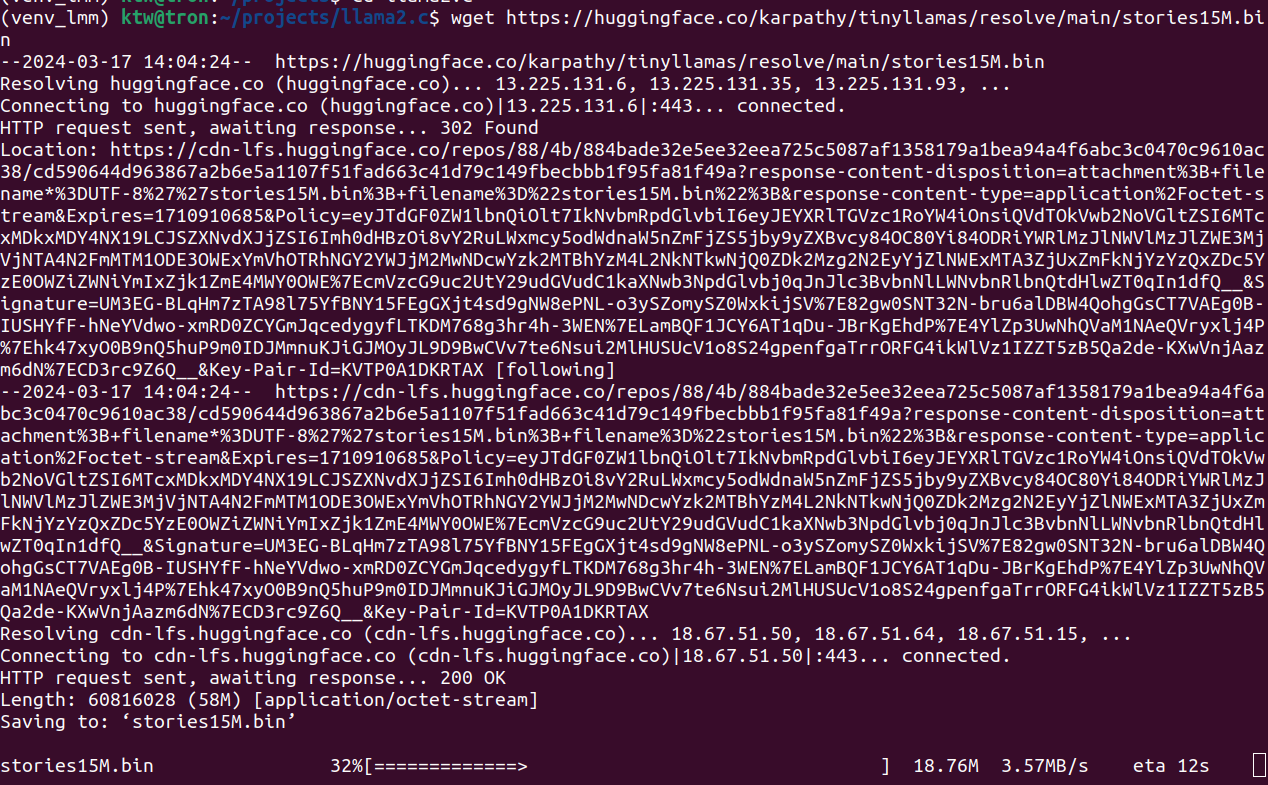
이제, 다음과 같이 하습 데이터셋 다운로드 코딩한다. 
from huggingface_hub import notebook_login  # 허깅페이스 모델 업로드 위한 임포트
notebook_login()

from datasets import load_dataset  # squad 데이터셋 다운로드
squad = load_dataset("squad", split="train[:5000]")
squad = squad.train_test_split(test_size=0.2)
print(squad['train'][0])

다음과 같이 토크나이저에 훈련 텍스트 입력 처리를 위해, 최대 길이를 절단하는 등의 처리 함수를 코딩한다.
from transformers import AutoTokenizer  #  distilbert 토큰나이저 임포트
tokenizer = AutoTokenizer.from_pretrained("distilbert/distilbert-base-uncased") 

def preprocess_function(examples):
    questions = [q.strip() for q in examples["question"]]
    inputs = tokenizer(
        questions,
        examples["context"],
        max_length=384,
        truncation="only_second",
        return_offsets_mapping=True,
        padding="max_length",
    )

    offset_mapping = inputs.pop("offset_mapping")
    answers = examples["answers"]
    start_positions = []
    end_positions = []

    for i, offset in enumerate(offset_mapping):
        answer = answers[i]
        start_char = answer["answer_start"][0]
        end_char = answer["answer_start"][0] + len(answer["text"][0])
        sequence_ids = inputs.sequence_ids(i)

        # Find the start and end of the context
        idx = 0
        while sequence_ids[idx] != 1:
            idx += 1
        context_start = idx
        while sequence_ids[idx] == 1:
            idx += 1
        context_end = idx - 1

        # If the answer is not fully inside the context, label it (0, 0)
        if offset[context_start][0] > end_char or offset[context_end][1] < start_char:
            start_positions.append(0)
            end_positions.append(0)
        else:
            # Otherwise it's the start and end token positions
            idx = context_start
            while idx <= context_end and offset[idx][0] <= start_char:
                idx += 1
            start_positions.append(idx - 1)

            idx = context_end
            while idx >= context_start and offset[idx][1] >= end_char:
                idx -= 1
            end_positions.append(idx + 1)

    inputs["start_positions"] = start_positions
    inputs["end_positions"] = end_positions
    return inputs

데이터셋을 앞의 정의된 함수로 전처리한다. 필요하지 않은 열은 제거한다. 
tokenized_squad = squad.map(preprocess_function, batched=True, remove_columns=squad["train"].column_names)

학습을 위해 배치를 만든다. 
from transformers import DefaultDataCollator
data_collator = DefaultDataCollator()

from transformers import AutoModelForQuestionAnswering, TrainingArguments, Trainer
model = AutoModelForQuestionAnswering.from_pretrained("distilbert/distilbert-base-uncased")  # 사전 학습 모델을 파인튜닝한다

training_args = TrainingArguments(
    output_dir="my_awesome_qa_model",
    evaluation_strategy="epoch",
    learning_rate=2e-5,
    per_device_train_batch_size=16,
    per_device_eval_batch_size=16,
    num_train_epochs=3,
    weight_decay=0.01,
    push_to_hub=True,
)  # 학습될 모델 및 파라메터 명시

trainer = Trainer(
    model=model,
    args=training_args,
    train_dataset=tokenized_squad["train"],
    eval_dataset=tokenized_squad["test"],
    tokenizer=tokenizer,
    data_collator=data_collator,
)  # 전이학습모델, 파라메터, 데이터셋, 토크나이져, 배치처리를 위한 데이터 컬렉터 설정

trainer.train()  # 학습
trainer.push_to_hub()  # 학습된 데이터를 허브에 업로드

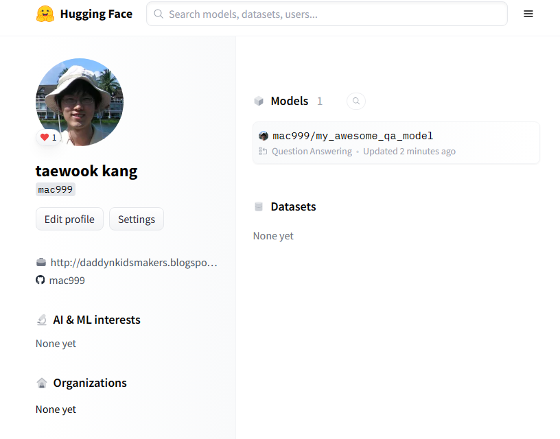
그 결과 다음과 같이 파인 튜닝된 학습 모델이 허브에 업로드되었다. 

다음과 같이 실행한다.
from transformers import pipeline

question = "How many programming languages does BLOOM support?"
context = "BLOOM has 176 billion parameters and can generate text in 46 languages natural languages and 13 programming languages."

question_answerer = pipeline("question-answering", model="my_awesome_qa_model")
question_answerer(question=question, context=context)

결과가 다음과 같다면 성공한 것이다.

NER(Named Entity Recognition) BERT 모델 파인튜닝
각 문장의 토큰 엔티티 의미를 인식하는 모델을 NER이라 한다. 문장 토큰의 의미를 인식할 수 있다면, 문장에서 특정 토큰에 대한 의미를 알고, 해당 의미에 대한 에이전트를 자동 실행하는 등의 서비스를 쉽게 개발할 수 있다. 

코드 개발 전에 다음을 설치한다. 
pip install transformers[torch] datasets

이 예제는 NER 데이터셋을 다운로드하고, BERT-BASE-NER(참고) 사전학습모델을 이용해 파인튜닝한다. BERT-BASE-NER 모델 사용방법은 다음과 같다. 
from transformers import AutoTokenizer, AutoModelForTokenClassification
from transformers import pipeline

tokenizer = AutoTokenizer.from_pretrained("dslim/bert-base-NER")
model = AutoModelForTokenClassification.from_pretrained("dslim/bert-base-NER")

nlp = pipeline("ner", model=model, tokenizer=tokenizer)
example = "My name is Wolfgang and I live in Berlin"

ner_results = nlp(example)
print(ner_results)

파인튜닝 데이터셋은 희귀한 토큰 의미를 정의한 데이터셋이다. 
NER 의미는 다음과 같다. 
Person
Location (including GPE, facility)
Corporation
Consumer good (tangible goods, or well-defined services)
Creative work (song, movie, book, and so on)
Group (subsuming music band, sports team, and non-corporate organisations)

이는 코드 상해 좀 더 상세화되어 표현되었다.
0: O
1: B-corporation
2: I-corporation
3: B-creative-work
4: I-creative-work
5: B-group
6: I-group
7: B-location
8: I-location
9: B-person
10: I-person
11: B-product
12: I-product

각 B, I, O는 Begin location, Inside location, Outside를 의미한다(NER 연구에 자주 나오는 용어). 참고로, New York City is a bustling metropolis의 NER 해석은 다음과 같다. 
New: O (Outside of any named entity)
York: B-LOC (Beginning of a Location entity)
City: I-LOC (Inside of a Location entity)
is: O
a: O
bustling: O
metropolis: O 

사용된 데이터셋은 다음과 같이 문장 토큰에 대한 NER이 정의되어 있다. 

이제, 다음 파인튜닝 코드를 입력해 실행, 학습한다. 
from transformers import AutoTokenizer
tokenizer = AutoTokenizer.from_pretrained("dslim/bert-base-NER")
def tokenize_and_align_tags(records):
    # 입력 단어를 토큰으로 분리함. 예를 들어, ChatGPT경우, ['Chat', '##G', '##PT']로 분해
    tokenized_results = tokenizer(records["tokens"], truncation=True, is_split_into_words=True)
    input_tags_list = []

    for i, given_tags in enumerate(records["ner_tags"]):
        word_ids = tokenized_results.word_ids(batch_index=i)
        previous_word_id = None
        input_tags = []

        for wid in word_ids:
            if wid is None:
                input_tags.append(-100)
            elif wid != previous_word_id:
                input_tags.append(given_tags[wid])
            else:
                input_tags.append(-100)
            previous_word_id = wid

        input_tags_list.append(input_tags)

    tokenized_results["labels"] = input_tags_list
    return tokenized_results

from datasets import load_dataset
wnut = load_dataset('wnut_17')
tokenized_wnut = wnut.map(tokenize_and_align_tags, batched=True)
tag_names = wnut["test"].features[f"ner_tags"].feature.names
id2label = dict(enumerate(tag_names))
label2id = dict(zip(id2label.values(), id2label.keys()))

from transformers import AutoModelForTokenClassification
model = AutoModelForTokenClassification.from_pretrained(
    "dslim/bert-base-NER", num_labels=len(id2label), id2label=id2label, label2id=label2id, ignore_mismatched_sizes=True
)

from transformers import Trainer, TrainingArguments, DataCollatorForTokenClassification
training_args = TrainingArguments(
    output_dir="my_finetuned_wnut_model",
)
''' # 하이퍼파라메터 튜닝용
training_args = TrainingArguments(
    output_dir="my_finetuned_wnut_model_1012",
    learning_rate=2e-5,
    per_device_train_batch_size=16,
    per_device_eval_batch_size=16,
    num_train_epochs=2,
    weight_decay=0.01,
    evaluation_strategy="epoch",
    save_strategy="epoch",
    load_best_model_at_end=True,
    push_to_hub=True,
)'''
data_collator = DataCollatorForTokenClassification(tokenizer=tokenizer)     
trainer = Trainer(
    model=model,
    args=training_args,
    train_dataset=tokenized_wnut["train"],
    eval_dataset=tokenized_wnut["test"],
    tokenizer=tokenizer,
    data_collator=data_collator,
)

trainer.train()

from transformers import pipeline
model = AutoModelForTokenClassification.from_pretrained("my_finetuned_wnut_model/checkpoint-1000")
tokenizer = AutoTokenizer.from_pretrained("my_finetuned_wnut_model/checkpoint-1000")

classifier = pipeline("ner", model=model, tokenizer=tokenizer)
out = classifier("My name is Sylvain and I work at Hugging Face in Brooklyn.")
print(out)

import evaluate
seqeval = evaluate.load("seqeval")
results = trainer.evaluate()
print(results)
trainer.push_to_hub()

실행 결과는 다음과 같다. 

다음과 같이 문장 각 토큰의 의미(예. 사람, 위치 등)를 높은 정확도로 제공해 준다. 

마무리
이 글은 허깅페이스 트랜스포머를 이용해 다양한 사전학습 모델을 이용해 여러가지 서비스 개발 방법을 살펴보았다. 자체 데이터로 학습하거나, 데이터 학습을 좀 더 많이 할 수록 결과가 더 정확하고, 전문적이며, 풍부해 질 것이다.

레퍼런스

2024년 3월 16일 토요일

GPU 없는 로컬에서 서비스 가능한 경량 소형 LLM, LLAMA2.c 빌드, 실행, 학습 및 코드 분석하기

이 글은 GPU 없는 컴퓨터에서 경량 LLAMA2.c (라마씨)를 빌드하고, 로컬에서 실행, 학습하는 방법을 간략히 따라해 본다.
LLAMA2.c

머리말
앞서 설명한 코드 라마2는 최소 28GB이상의 GPU RAM이 필요하다. 많은 개발자의 경우, 현재 시점에서 이 정도 수준의 GPU 스펙 장비를 가진 경우는 매우 드물다. CoLab의 경우 T4 GPU는 16GB 크기를 가진다. 그러므로, 이를 해결할 수 있는 솔류션이 개발되었다. 

LLAMA2.c는 OpenAI 엔지니어인 Andrej Karpathy가 개발한 라마2를 이용한 소형 LLM 오픈소스 프로젝트이다. 이 라마 코드는 순수 C로 개발되었으며, 모델은 겨우 100MB로 동작되어, GPU가 없는 로컬 PC에서도 가볍게 실행된다. 

LLAMA.c 설치
설치, 실행 및 학습 방법은 다음과 같다. 터미널에서 다음 명령을 실행한다.
cd llama2.c
wget https://huggingface.co/karpathy/tinyllamas/resolve/main/stories15M.bin

이 결과, https://huggingface.co/datasets/roneneldan/TinyStories 으로 학습된 모델이 다운로드된다.

실행하기
코드를 컴파일하고, 다운로드받은 스토리 학습 모델을 실행한다. 
make run
./run stories15M.bin

실행 결과는 다음과 같다. 텍스트가 잘 생성되는 것을 확인할 수 있다.

좀 더 큰 모델을 다운받아 실행해 본다.
wget https://huggingface.co/karpathy/tinyllamas/resolve/main/stories42M.bin
./run stories42M.bin
./run stories42M.bin -t 0.8 -n 256 -i "One day, Lily met a Shoggoth"


다음과 같이, 접두어, 추가 명령줄 인수를 지정할 수도 있다.
-t: 생성 온도. 0~1.0
 
데이터 학습 방법
새로운 데이터 훈련을 위해서는 앞에서 사용한 스토리 모델이 어떻게 학습되었는지 확인해 볼 필요가 있다. 그 방법은 다음과 같다.
python tinystories.py download
python tinystories.py pretokenize
python train.py

학습 데이터 다운로드 화면 일부

이제 컴파일을 한다. 
make run

다음과 같이 실행하면 된다. 
./run stories15M.bin

코드 및 학습 데이터 분석하기
LLAMA2.c의 구조는 매우 간단한데, make파일을 분석해 보면 단 하나의 run.c를 컴파일해 실행파일을 빌드하는 것을 확인할 수 있다.
gcc -O3 -o run run.c -lm

run.c의 주요 부분을 살펴보면 다음과 같다. 
typedef struct {
    // token embedding table
    float* token_embedding_table;    // (vocab_size, dim)
    // weights for rmsnorms
    float* rms_att_weight; // (layer, dim) rmsnorm weights
    float* rms_ffn_weight; // (layer, dim)
    // weights for matmuls. note dim == n_heads * head_size
    float* wq; // (layer, dim, n_heads * head_size)
    float* wk; // (layer, dim, n_kv_heads * head_size)
    float* wv; // (layer, dim, n_kv_heads * head_size)
    float* wo; // (layer, n_heads * head_size, dim)
    // weights for ffn
    float* w1; // (layer, hidden_dim, dim)
    float* w2; // (layer, dim, hidden_dim)
    float* w3; // (layer, hidden_dim, dim)
    // final rmsnorm
    float* rms_final_weight; // (dim,)
    // (optional) classifier weights for the logits, on the last layer
    float* wcls;
} TransformerWeights;

이 구조체의 이름은 TransformerWeights이며, 이는 Transformer 모델의 가중치를 저장하는 데 사용된다. 트랜스포머의 어텐션 스코어를 계산하는 데 핵심적인 자료구조이다. 각 필드는 다음과 같은 의미를 가진다:
  • token_embedding_table: 토큰 임베딩 테이블을 나타낸다. 이는 어휘 크기(vocab_size)와 차원(dim)의 2차원 배열이다.
  • rms_att_weight, rms_ffn_weight: RMSNorm의 가중치를 나타낸다. 각각 attention과 feed-forward network에 대한 것이다.
  • wq, wk, wv, wo: 각각 query, key, value, output에 대한 가중치를 나타낸다. 이들은 multi-head attention에서 사용된다.
  • w1, w2, w3: feed-forward network에서 사용되는 가중치이다.
  • rms_final_weight: 최종 RMSNorm의 가중치를 나타낸다.
  • wcls: (선택적으로) 마지막 레이어에서 로짓에 대한 분류기 가중치를 나타낸다.
  • 이 구조체는 Transformer 모델의 가중치를 저장하고 관리하는 데 사용된다.
전체적인 프로그램 실행 구조는 다음과 같다. 

1. 이 코드는 트랜스포머 모델의 구성, 가중치 및 상태에 대한 구조와 메모리 할당, 메모리 해제 및 체크포인트 읽기 기능을 정의한다.
2. 'rmsnorm', 'softmax', 'matmul'과 같은 신경망 블록을 위한 함수도 포함되어 있다.
3. 코드는 Transformer 모델을 통해 입력 토큰을 처리하여 출력 로짓을 생성하는 'forward' 함수를 구현한다.
4. 또한 BPE(Byte Pair Encoding) 토크나이저가 문자열을 토큰으로 또는 그 반대로 변환하는 구조와 함수가 있다.
5. 코드에는 argmax, 샘플링 및 top-p 샘플링과 같은 다양한 전략을 사용하여 확률을 기반으로 토큰을 샘플링하는 '샘플러' 구조와 함수가 포함된다.
6. 시간 측정을 위한 유틸리티 기능과 Transformer 모델을 기반으로 텍스트를 생성하는 '생성' 기능을 정의한다.
7. 마지막으로 트랜스포머 모델을 사용하여 사용자와 어시스턴트 간의 대화를 시뮬레이션하는 '채팅' 기능을 정의한다.  
전체 프로그램 구조도

앞에서 사용된 1.5GB가 넘는 스토리 학습 데이터의 구조는 다음과 같이 되어 있다.
학습 데이터 구조 일부

이를 본인의 목적에 맞게 적절히 데이터를 준비한 후, 다음과 같이 동일한 방식으로 학습하면 가중치 벡터가 저장된 bin파일을 얻을 수 있다. 이를 이용해, 앞서 언급된 방식과 동일하게 사용하면 된다.

레퍼런스